.png)
Conducted Emissions
- Dario Fresu

- Nov 19, 2024
- 17 min read
Updated: Mar 31

Conducted Emissions
In this lesson, we’ll dive into the world of conducted emissions, what causes them, how they affect your circuits, and, most importantly, proven strategies to mitigate these issues right from the Printed Circuit Board Design.
Conducted emissions are simply radiated emissions in disguise.
The simple reason for dividing them into conducted and radiated emissions is that it makes testing easier.
The problem with measuring emissions below 30MHz using the same testing methodology as radiated emissions is that the wavelengths of the signals can be in the near-field region, leading to results that do not match reality.
If we measure emissions above 30MHz using the same testing methodology as the conducted emissions test, we encounter a different issue: the cable can start to resonate at these frequencies, which will also yield incorrect results.
The main objective of the conductive emissions tests, is to ensure that the emission levels are under certain thresholds. This is because if disturbances find a way to escape from the system, they may potentially spread around and upset other systems.
One common way for this to occur, if left uncontrolled, is when disturbances are conducted out of the systems through the power cords.
What can happen in this scenario is that the conducted disturbance, through the power cord, may reach the power distribution system. This is quite important because the structure of the power distribution system is built in a way that resembles a large antenna structure, which can potentially radiate and upset many other systems that can be susceptible to that.
To aggravate the issue, since the power distribution network is built with long cables, this gives the possibility for large wavelengths to find a radiative structure and potentially radiate.
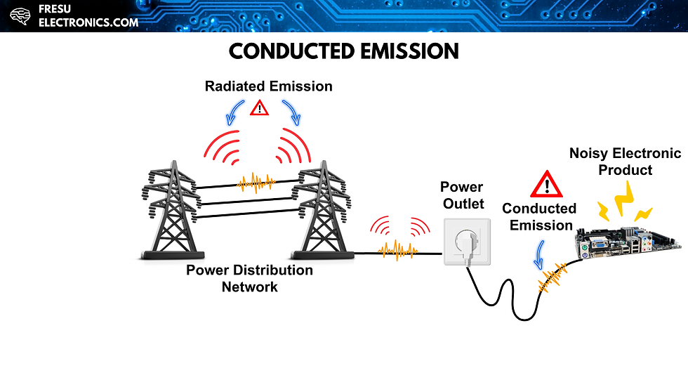
This is why regulatory bodies, like the FCC and the CISPR, impose limits on these emissions, so that we create an environment with fewer emission pollutants, where systems can instead work in harmony with each other.
Susceptibility or Immunity
In the same way, we want to prevent not only that our system has limited emission levels, but also that its susceptibility, or immunity to these emissions, is controlled, providing robustness for our system.
One of the most common ways susceptibility or immunity issues arise is through disturbances reaching our system, such as lightning strikes on the power transmission lines providing power to the installation.
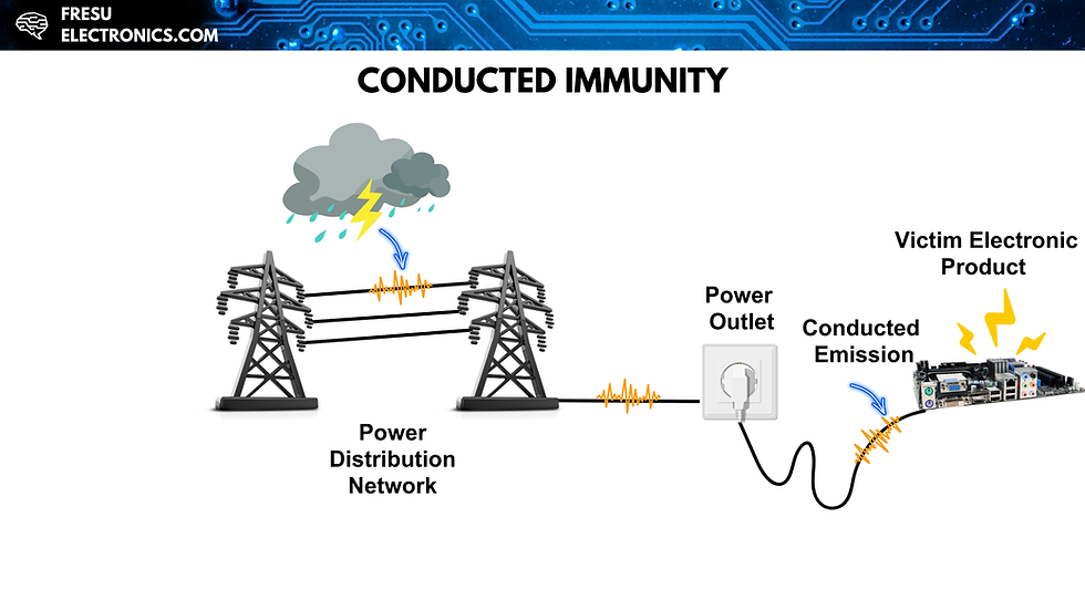
Some of these disturbances may also cause the loss of power for long periods or short temporary outages. In the former case, the systems are not expected to maintain operation.
However, in the latter case, for example when the circuit breaker is attempting to reestablish power, the product is expected to maintain normal operation without loss of data or function.
Testing
In order to test the systems, and verify that their level of emissions is within a certain safe range, regulatory agencies such as the FCC and CISPR have established limits with which systems must comply.
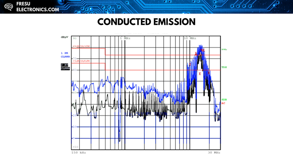
A typical range of frequencies to which the systems are tested against in conducted emission tests is from 150 kHz to 30 MHz. However, this limit may vary depending on the specific standards that the system has to comply with.
Within this range of frequencies, the FCC and CISPR have specific requirements to be met for different ranges of frequencies.
Conducted emissions are classified into different categories based on their frequency range and the standards they comply with. The most common classes for conducted emissions are: Class A, and Class B.
Class A:
This class typically applies to industrial environments where there are fewer restrictions on emissions. Devices in this class have emissions limits set at higher levels compared to Class B.
Class B:
Devices in this class need to meet stricter emissions limits. This is important for devices used in residential or commercial settings where there is a need to minimize interference.
These classes, help ensure that electronic devices meet specific emission standards, depending on their intended use, and the environment in which they will be operating.
For Class A digital devices: The quasy peak limit is of 79 dBuV, from 150 kHz to 500 kHz. And then from 500 kHz to 30 MHz, the quasy peak limit is of 73 dBuV.
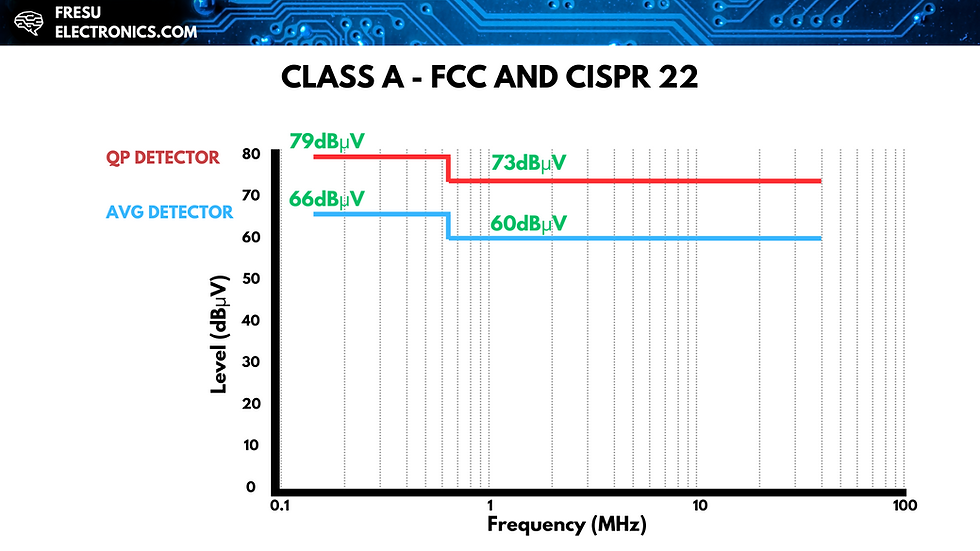
For the average limit, the light blue line, the limits are set to 66 dBuV and is from 150 kHz to 500 kHz. And then from 500 kHz to 30 MHz, the average peak limit is of 60dBuV.
For Class-B digital devices: The quasy peak limit goes from 66 dBuV to 56, from 150 kHz to 500 kHz. And then from 500 kHz to 5 MHz, the quasy peak limit is of 56 dBuV. To then again increase to 60 dBuV from 5 MHz to 30 MHz.

For the average limit, the light blue line, the limit goes from 56 dBuV to 46, from 150 kHz to 500 kHz. And then from 500 kHz to 5 MHz, the quasy peak limit is of 46 dBuV. To then again increase to 50 dBuV from 5 MHz to 30 MHz.
A common approach when doing pre-compliance testing, before going to the certifying EMC lab, is to keep the system's emissions at least 6 dB below the required limits.
Want to read more?
Subscribe to fresuelectronics.com to keep reading this exclusive post.